NanoNeuron - 7 simple JS functions that explain how machines learn
TL;DR
NanoNeuron is an over-simplified version of the Neuron concept from Neural Networks. NanoNeuron is trained to convert temperature values from Celsius to Fahrenheit.
The NanoNeuron.js code example contains 7 simple JavaScript functions (which touches on model prediction, cost calculation, forward/backwards propagation, and training) that will give you a feeling of how machines can actually "learn". No 3rd-party libraries, no external data-sets or dependencies, only pure and simple JavaScript functions.
☝🏻These functions are NOT, by any means, a complete guide to machine learning. A lot of machine learning concepts are skipped and over-simplified! This simplification is done on purpose to give the reader a really basic understanding and feeling of how machines can learn and ultimately to make it possible for the reader to recognize that it's not "machine learning MAGIC" but rather "machine learning MATH" 🤓.
What our NanoNeuron will learn
You've probably heard about Neurons in the context of Neural Networks. NanoNeuron is just that but simpler and we're going to implement it from scratch. For simplicity reasons we're not even going to build a network on NanoNeurons. We will have it all working on its own, doing some magical predictions for us. Namely, we will teach this singular NanoNeuron to convert (predict) the temperature from Celsius to Fahrenheit.
By the way, the formula for converting Celsius to Fahrenheit is this:
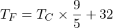
But for now our NanoNeuron doesn't know about it...
The NanoNeuron model
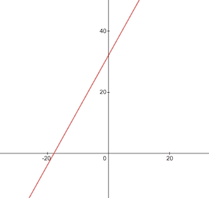
Let's implement our NanoNeuron model function. It implements basic linear dependency between x and y which looks like y = w * x + b. Simply saying our NanoNeuron is a "kid" in a "school" that is being taught to draw the straight line in XY coordinates.
Variables w, b are parameters of the model. NanoNeuron knows only about these two parameters of the linear function.
These parameters are something that NanoNeuron is going to "learn" during the training process.
The only thing that NanoNeuron can do is to imitate linear dependency. In its predict() method it accepts some input x and predicts the output y. No magic here.
function NanoNeuron(w, b) {
  this.w = w;
  this.b = b;
  this.predict = (x) => {
    return x * this.w + this.b;
  }
}
...wait... linear regression is it you? 🧐
Celsius to Fahrenheit conversion
The temperature value in Celsius can be converted to Fahrenheit using the following formula: f = 1.8 * c + 32, where c is a temperature in Celsius and f is the calculated temperature in Fahrenheit.
function celsiusToFahrenheit(c) {
  const w = 1.8;
  const b = 32;
  const f = c * w + b;
  return f;
};
Ultimately we want to teach our NanoNeuron to imitate this function (to learn that w = 1.8 and b = 32) without knowing these parameters in advance.
This is how the Celsius to Fahrenheit conversion function looks like:
Generating data-sets
Before the training we need to generate training and test data-sets based on the celsiusToFahrenheit() function. Data-sets consist of pairs of input values and correctly labeled output values.
In real life, in most of cases, this data would be collected rather than generated. For example, we might have a set of images of hand-drawn numbers and the corresponding set of numbers that explains what number is written on each picture.
We will use TRAINING example data to train our NanoNeuron. Before our NanoNeuron will grow and be able to make decisions on its own, we need to teach it what is right and what is wrong using training examples.
We will use TEST examples to evaluate how well our NanoNeuron performs on the data that it didn't see during the training. This is the point where we could see that our "kid" has grown and can make decisions on its own.
function generateDataSets() {
  // xTrain -> [0, 1, 2, ...],
  // yTrain -> [32, 33.8, 35.6, ...]
  const xTrain = [];
  const yTrain = [];
  for (let x = 0; x < 100; x += 1) {
    const y = celsiusToFahrenheit(x);
    xTrain.push(x);
    yTrain.push(y);
  }

  // xTest -> [0.5, 1.5, 2.5, ...]
  // yTest -> [32.9, 34.7, 36.5, ...]
  const xTest = [];
  const yTest = [];
  // By starting from 0.5 and using the same step of 1 as we have used for training set
  // we make sure that test set has different data comparing to training set.
  for (let x = 0.5; x < 100; x += 1) {
    const y = celsiusToFahrenheit(x);
    xTest.push(x);
    yTest.push(y);
  }

  return [xTrain, yTrain, xTest, yTest];
}
The cost (the error) of prediction
We need to have some metric that will show us how close our model's prediction is to correct values. The calculation of the cost (the mistake) between the correct output value of y and prediction, that our NanoNeuron created, will be made using the following formula:
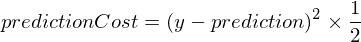
This is a simple difference between two values. The closer the values are to each other, the smaller the difference. We're using a power of 2 here just to get rid of negative numbers so that (1 - 2) ^ 2 would be the same as (2 - 1) ^ 2. Division by 2 is happening just to simplify further the backward propagation formula (see below).
The cost function in this case will be as simple as:
function predictionCost(y, prediction) {
  return (y - prediction) ** 2 / 2; // i.e. -> 235.6
}
Forward propagation
To do forward propagation means to do a prediction for all training examples from xTrain and yTrain data-sets and to calculate the average cost of those predictions along the way.
We just let our NanoNeuron say its opinion, at this point, by just allowing it to guess how to convert the temperature. It might be stupidly wrong here. The average cost will show us how wrong our model is right now. This cost value is really important since changing the NanoNeuron parameters w and b, and by doing the forward propagation again; we will be able to evaluate if our NanoNeuron became smarter or not after these parameters change.
The average cost will be calculated using the following formula:
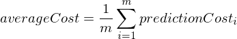
Where m is a number of training examples (in our case: 100).
Here is how we may implement it in code:
function forwardPropagation(model, xTrain, yTrain) {
  const m = xTrain.length;
  const predictions = [];
  let cost = 0;
  for (let i = 0; i < m; i += 1) {
    const prediction = nanoNeuron.predict(xTrain[i]);
    cost += predictionCost(yTrain[i], prediction);
    predictions.push(prediction);
  }
  // We are interested in average cost.
  cost /= m;
  return [predictions, cost];
}
Backward propagation
When we know how right or wrong our NanoNeuron's predictions are (based on average cost at this point) what should we do to make the predictions more precise?
The backward propagation gives us the answer to this question. Backward propagation is the process of evaluating the cost of prediction and adjusting the NanoNeuron's parameters w and b so that next and future predictions would be more precise.
This is the place where machine learning looks like magic 🧞♂️. The key concept here is the derivative which shows what step to take to get closer to the cost function minimum.
Remember, finding the minimum of a cost function is the ultimate goal of the training process. If we find such values for w and b such that our average cost function will be small, it would mean that the NanoNeuron model does really good and precise predictions.
Derivatives are a big and separate topic that we will not cover in this article. MathIsFun is a good resource to get a basic understanding of it.
One thing about derivatives that will help you to understand how backward propagation works is that the derivative, by its meaning, is a tangent line to the function curve that points toward the direction of the function minimum.

Image source: MathIsFun
For example, on the plot above, you can see that if we're at the point of (x=2, y=4) then the slope tells us to go left and down to get to the function minimum. Also notice that the bigger the slope, the faster we should move to the minimum.
The derivatives of our averageCost function for parameters w and b looks like this:
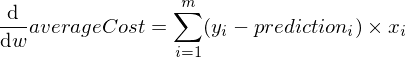
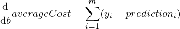
Where m is a number of training examples (in our case: 100).
You may read more about derivative rules and how to get a derivative of complex functions here.
function backwardPropagation(predictions, xTrain, yTrain) {
  const m = xTrain.length;
  // At the beginning we don't know in which way our parameters 'w' and 'b' need to be changed.
  // Therefore we're setting up the changing steps for each parameters to 0.
  let dW = 0;
  let dB = 0;
  for (let i = 0; i < m; i += 1) {
    dW += (yTrain[i] - predictions[i]) * xTrain[i];
    dB += yTrain[i] - predictions[i];
  }
  // We're interested in average deltas for each params.
  dW /= m;
  dB /= m;
  return [dW, dB];
}
Training the model
Now we know how to evaluate the correctness of our model for all training set examples (forward propagation). We also know how to do small adjustments to parameters w and b of our NanoNeuron model (backward propagation). But the issue is that if we run forward propagation and then backward propagation only once, it won't be enough for our model to learn any laws/trends from the training data. You may compare it with attending a one day of elementary school for the kid. He/she should go to the school not once but day after day and year after year to learn something.
So we need to repeat forward and backward propagation for our model many times. That is exactly what the trainModel() function does. It is like a "teacher" for our NanoNeuron model:
- it will spend some time (
epochs) with our slightly stupid NanoNeuron model and try to train/teach it, - it will use specific "books" (
xTrainandyTraindata-sets) for training, - it will push our kid to learn harder (faster) by using a learning rate parameter
alpha
A few words about the learning rate alpha. This is just a multiplier for dW and dB values we have calculated during the backward propagation. So, derivative pointed us toward the direction we need to take to find a minimum of the cost function (dW and dB sign) and it also showed us how fast we need to go in that direction (absolute values of dW and dB). Now we need to multiply those step sizes to alpha just to adjust our movement to the minimum faster or slower. Sometimes if we use big values for alpha, we might simply jump over the minimum and never find it.
The analogy with the teacher would be that the harder s/he pushes our "nano-kid" the faster our "nano-kid" will learn but if the teacher pushes too hard, the "kid" will have a nervous breakdown and won't be able to learn anything 🤯.
Here is how we're going to update our model's w and b params:

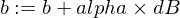
Here is our trainer function:
function trainModel({model, epochs, alpha, xTrain, yTrain}) {
  // The is the history array of how NanoNeuron learns.
  const costHistory = [];

  // Let's start counting epochs.
  for (let epoch = 0; epoch < epochs; epoch += 1) {
    // Forward propagation.
    const [predictions, cost] = forwardPropagation(model, xTrain, yTrain);
    costHistory.push(cost);

    // Backward propagation.
    const [dW, dB] = backwardPropagation(predictions, xTrain, yTrain);

    // Adjust our NanoNeuron parameters to increase accuracy of our model predictions.
    nanoNeuron.w += alpha * dW;
    nanoNeuron.b += alpha * dB;
  }

  return costHistory;
}
Putting all the pieces together
Now let's use the functions we have created above.
Let's create our NanoNeuron model instance. At this moment the NanoNeuron doesn't know what values should be set for parameters w and b. So let's set up w and b randomly.
const w = Math.random(); // i.e. -> 0.9492
const b = Math.random(); // i.e. -> 0.4570
const nanoNeuron = new NanoNeuron(w, b);
Generate training and test data-sets.
const [xTrain, yTrain, xTest, yTest] = generateDataSets();Let's train the model with small incremental (0.0005) steps for 70000 epochs. You can play with these parameters, they are being defined empirically.
const epochs = 70000;
const alpha = 0.0005;
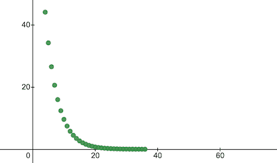
const trainingCostHistory = trainModel({model: nanoNeuron, epochs, alpha, xTrain, yTrain});Let's check how the cost function was changing during the training. We're expecting that the cost after the training should be much lower than before. This would mean that NanoNeuron got smarter. The opposite is also possible.
console.log('Cost before the training:', trainingCostHistory[0]); // i.e. -> 4694.3335043
console.log('Cost after the training:', trainingCostHistory[epochs - 1]); // i.e. -> 0.0000024
This is how the training cost changes over the epochs. On the x axes is the epoch number x1000.
Let's take a look at NanoNeuron parameters to see what it has learned. We expect that NanoNeuron parameters w and b to be similar to ones we have in the celsiusToFahrenheit() function (w = 1.8 and b = 32) since our NanoNeuron tried to imitate it.
console.log('NanoNeuron parameters:', {w: nanoNeuron.w, b: nanoNeuron.b}); // i.e. -> {w: 1.8, b: 31.99}Evaluate the model accuracy for the test data-set to see how well our NanoNeuron deals with new unknown data predictions. The cost of predictions on test sets is expected to be close to the training cost. This would mean that our NanoNeuron performs well on known and unknown data.
[testPredictions, testCost] = forwardPropagation(nanoNeuron, xTest, yTest);
console.log('Cost on new testing data:', testCost); // i.e. -> 0.0000023
Now, since we see that our NanoNeuron "kid" has performed well in the "school" during the training and that he can convert Celsius to Fahrenheit temperatures correctly, even for the data it hasn't seen, we can call it "smart" and ask him some questions. This was the ultimate goal of the entire training process.
const tempInCelsius = 70;
const customPrediction = nanoNeuron.predict(tempInCelsius);
console.log(`NanoNeuron "thinks" that ${tempInCelsius}°C in Fahrenheit is:`, customPrediction); // -> 158.0002
console.log('Correct answer is:', celsiusToFahrenheit(tempInCelsius)); // -> 158
So close! As all of us humans, our NanoNeuron is good but not ideal :)
Happy learning to you!
How to launch NanoNeuron
You may clone the repository and run it locally:
git clone https://github.com/trekhleb/nano-neuron.git
cd nano-neuron
node ./NanoNeuron.jsSkipped machine learning concepts
The following machine learning concepts were skipped and simplified for simplicity of explanation.
Training/testing data-set splitting
Normally you have one big set of data. Depending on the number of examples in that set, you may want to split it in proportion of 70/30 for train/test sets. The data in the set should be randomly shuffled before the split. If the number of examples is big (i.e. millions) then the split might happen in proportions that are closer to 90/10 or 95/5 for train/test data-sets.
The network brings the power
Normally you won't notice the usage of just one standalone neuron. The power is in the network of such neurons. The network might learn much more complex features. NanoNeuron alone looks more like a simple linear regression than a neural network.
Input normalization
Before the training, it would be better to normalize input values.
Vectorized implementation
For networks, the vectorized (matrix) calculations work much faster than for loops. Normally forward/backward propagation works much faster if it is implemented in vectorized form and calculated using, for example, Numpy Python library.
Minimum of the cost function
The cost function that we were using in this example is over-simplified. It should have logarithmic components. Changing the cost function will also change its derivatives so the back propagation step would also use different formulas.
Activation function
Normally the output of a neuron should be passed through an activation function like Sigmoid or ReLU or others.
Subscribe to the Newsletter
Get my latest posts and project updates by email